Hamiltonian Monte Carlo from scratch, in NumPy and JAX
Hamiltonian Monte Carlo has a beautiful idea at its core: instead of proposing random steps and hoping for the best, let the gradient of your log-density guide the sampler like a particle rolling through an energy landscape. The physics does real work. The problem is the gradient.
For any moderately complex model, getting that gradient is the entire computational bottleneck. Derive it analytically and you spend an afternoon with pencil and paper for every new likelihood, one sign error away from a sampler that looks correct and isn’t. Use finite differences and you pay two full log-density evaluations per parameter per leapfrog step. At 50 parameters, that is 100 evaluations per step, 2000 per proposal. The cost grows linearly with dimension and there is no way around it.
As an astrophysicist fitting high-dimensional models to spectral data, I got tired of both options. JAX’s jax.grad eliminates the choice: write your log-density once with jnp.* primitives and you get the exact gradient for any model, regardless of its structure, at the cost of a single backward pass.
This post builds HMC from scratch twice. First in NumPy with finite differences, to feel the bottleneck. Then in JAX, to see it disappear. The code is in the JaxHMC repository.
1. A little 19th-century physics for your posteriors
The core of HMC is a beautiful reinterpretation: your target distribution is a potential energy landscape. The probability mass concentrates in the valleys, the tails stretch up the hillsides, and sampling from $\pi$ is equivalent to simulating a particle rolling around on that landscape without friction.
More precisely, define the potential energy as the negative log-density of your target:
\[U(q) = -\log \pi(q)\]where $q \in \mathbb{R}^d$ is the parameter vector you want to sample. Regions of high probability correspond to low potential energy, exactly like physical valleys. Now introduce an auxiliary momentum variable $p \in \mathbb{R}^d$, drawn fresh at each step from an independent Gaussian. This momentum carries the particle and allows it to climb hills it could never reach by diffusion alone. The kinetic energy is the standard quadratic form:
\[K(p) = \frac{1}{2} p^\top M^{-1} p\]where $M$ is a mass matrix (often just $I$ to start). The mass matrix $M$ preconditions the momentum: when $M \approx \Sigma$ (the posterior covariance), the kinetic energy is adapted to the posterior geometry and the leapfrog takes balanced steps in all directions. Using $M = I$ on a poorly conditioned posterior forces a step size calibrated to the narrowest direction, wasting the broader dimensions. Modern implementations estimate $M$ during warmup. Their sum is the total energy, the Hamiltonian:
\[H(q, p) = U(q) + K(p) = -\log \pi(q) + \frac{1}{2} p^\top M^{-1} p\]The joint distribution over position and momentum is
\[\pi(q, p) \propto \exp(-H(q, p)) = \pi(q) \cdot \mathcal{N}(p \mid 0, M)\]which is just the target marginalised by an independent Gaussian on $p$. If we can sample from the joint distribution, we get samples from the target for free by discarding $p$.
Now here is where the physics does the work. Hamiltonian dynamics are governed by Hamilton’s equations:
\[\frac{dq}{dt} = \frac{\partial H}{\partial p} = M^{-1}p, \qquad \frac{dp}{dt} = -\frac{\partial H}{\partial q} = -\nabla U(q)\]These equations have a remarkable property: they conserve the Hamiltonian exactly. A particle obeying these equations moves through phase space $(q, p)$ while keeping $H$ constant. In terms of probability, this means the particle is moving along iso-density surfaces of $\pi(q, p)$, always in high-probability territory, never drifting away from the mass.
This is the reason HMC works. A random-walk Metropolis proposal is blind: it does not know whether the proposed point is in a high-density region until it evaluates the density there. An HMC proposal follows a deterministic trajectory that, if simulated exactly, would be accepted with probability one, because $H$ is perfectly conserved. In practice, we use a numerical integrator and $H$ is approximately conserved, so the acceptance rate is very high but not exactly one.
Hamiltonian dynamics are also time-reversible: if you flip the sign of all momenta and run the simulation backwards, you return exactly to your starting point. This reversibility is what ensures the Markov chain satisfies detailed balance and therefore has $\pi$ as its stationary distribution. Combined with the volume-preserving nature of the flow, the Liouville theorem guarantees that the phase-space volume element $dq\, dp$ is preserved. Together these properties yield a valid MCMC algorithm almost for free.
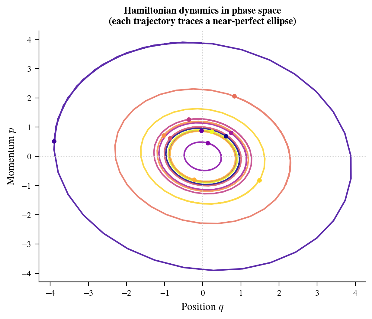 Figure 1: Leapfrog trajectories in phase space $(q, p)$ for a correlated Gaussian target. Each trajectory conserves the Hamiltonian (visible as constant-color level curves), demonstrating that proposals stay on iso-density surfaces. The particle slides around the energy contour rather than diffusing randomly.
The intuition to hold onto: instead of proposing a random step and hoping for the best, HMC proposes the endpoint of a physics simulation. The gradient of $U(q)$ tells the particle which way is downhill, and the momentum carries it forward with inertia. Steep gradients create fast, directed motion; gentle gradients allow long coasting trajectories. This is why HMC can explore high-dimensional posteriors in far fewer evaluations than a random walk.
2. The HMC algorithm
The physics of the previous section is ideal: continuous, exact, and energy-conserving. To turn it into a practical algorithm, we need to discretize Hamilton’s equations. The tool of choice is the leapfrog integrator, and the reasons for this specific choice are not arbitrary.
A naive Euler integration of Hamilton’s equations accumulates errors that grow exponentially, sending the particle spiraling off to infinity. The leapfrog avoids this by interleaving half-steps of momentum with full steps of position in a specific staggered pattern. The leapfrog is symplectic: it exactly conserves a shadow Hamiltonian $\tilde{H}$ that is close to the true $H$, differing by $O(\varepsilon^2)$. The energy error $\Delta H$ over an entire $L$-step trajectory stays $O(\varepsilon^2)$ and does not accumulate. Non-symplectic integrators (Euler, RK4) have no such bound: their energy error grows without a ceiling over long trajectories. Volume preservation (Liouville’s theorem) is a direct consequence of symplecticity and is equally essential for the MH acceptance step to be valid.
With a mass matrix $M = I$ (the identity, for simplicity), a single leapfrog trajectory of $L$ steps starting from $(q_0, p_0)$ proceeds as follows.
Half-step for momentum:
\[p_{1/2} = p_0 - \frac{\varepsilon}{2} \nabla U(q_0)\]Full steps: for $\ell = 1, \ldots, L-1$,
\[q_\ell = q_{\ell-1} + \varepsilon\, p_{\ell - 1/2}\] \[p_{\ell + 1/2} = p_{\ell - 1/2} - \varepsilon\, \nabla U(q_\ell)\]Final position update and half-step:
\[q_L = q_{L-1} + \varepsilon\, p_{L-1/2}\] \[p_L = p_{L-1/2} - \frac{\varepsilon}{2} \nabla U(q_L)\]This staggered structure (half-step, full-steps, half-step) is what gives the leapfrog its symplectic character. Think of it as the position and momentum taking turns: the gradient at $q$ updates $p$, the updated $p$ moves $q$, and so on, with the two halves of the momentum update bracketing each full position step.
After $L$ leapfrog steps, the proposal $(q_L, p_L)$ is evaluated with a standard Metropolis-Hastings acceptance step. The acceptance probability is:
\[\alpha = \min\!\left(1,\, e^{-\Delta H}\right), \quad \Delta H = H(q_L, p_L) - H(q_0, p_0)\]Because the leapfrog is nearly energy-conserving, $\Delta H \approx 0$ and acceptance rates are typically above 80–90%. The time-reversibility of the leapfrog ensures that the MH correction is valid: we can flip the sign of $p_L$ and use the same formula with the same measure.
Why HMC beats random-walk Metropolis. A random-walk proposal of step size $\delta$ moves a distance $O(\delta)$ per step and must keep $\delta$ small to maintain reasonable acceptance. To move a distance $D$ across the posterior, you need $O(D/\delta)^2$ steps (a diffusive, random-walk scaling). HMC with step size $\varepsilon$ and $L$ leapfrog steps proposes a move of distance $O(L\varepsilon)$ per accepted step, independently of the acceptance rate. By choosing $L\varepsilon \approx 1$ (roughly the typical scale of the posterior), you can traverse the distribution in $O(1)$ accepted steps rather than $O(D^2/\varepsilon^2)$. This improvement is not just a constant factor. For a $d$-dimensional posterior with independent components, random-walk MH requires $O(d)$ steps per independent sample, while HMC requires only $O(d^{1/4})$, a ratio growing as $d^{3/4}$ in HMC’s favor. (This result is from Neal (2011) and holds under specific regularity conditions; correlated and hierarchical posteriors can be harder.)
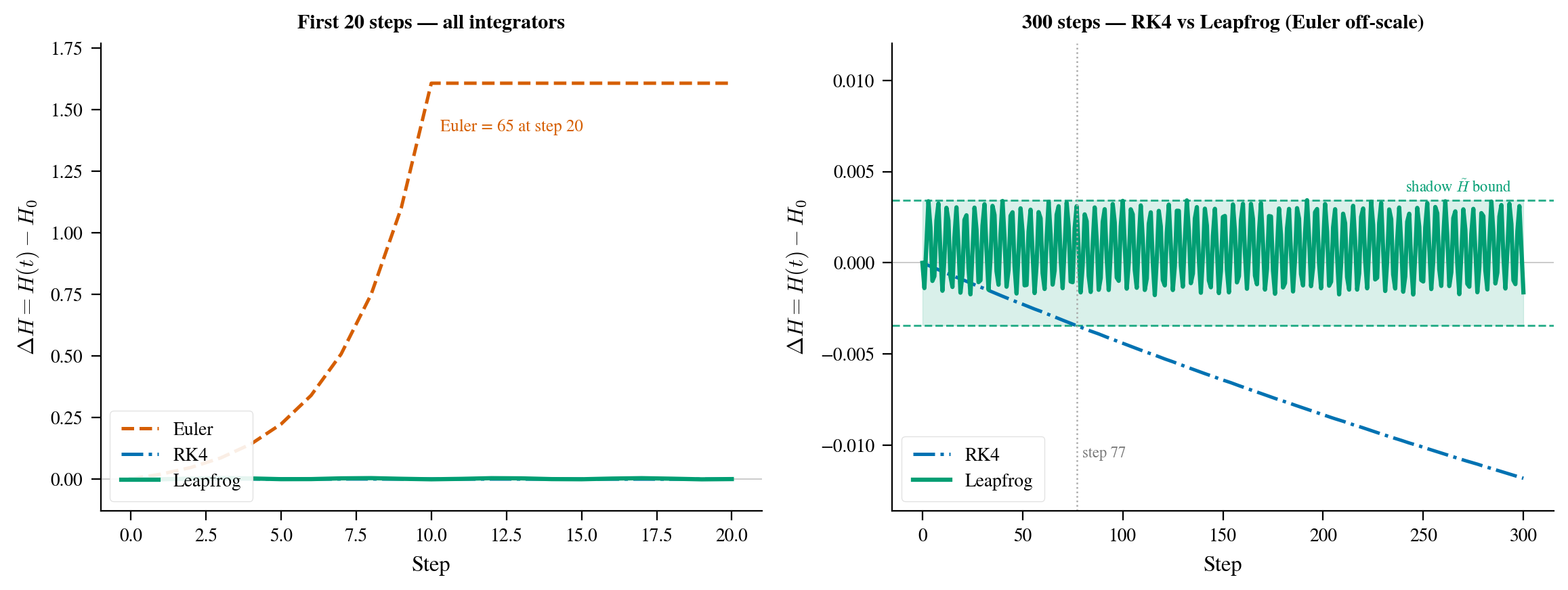 Figure 2: Energy error $\Delta H = H(t) - H_0$ on the banana distribution ($\varepsilon = 0.1$, 300 steps). Left: Euler exits the frame within the first few steps. Right: RK4 exhibits secular energy drift without bound, a signature of non-symplectic integration (the drift direction is system-specific). Leapfrog oscillates inside the green band and never leaves it. Those oscillations are not noise: leapfrog exactly conserves a shadow Hamiltonian $\tilde{H} = H + O(\varepsilon^2)$ slightly different from $H$, so $\Delta H = H - \tilde{H}$ bounces back and forth with a fixed amplitude proportional to $\varepsilon^2$, bounded forever. RK4 has no such conservation law. Its error grows without bound, which would slowly corrupt MCMC samples over long chains.
The two hyperparameters $\varepsilon$ (step size) and $L$ (number of steps) require tuning. $\varepsilon$ too large and the leapfrog error grows, leading to high rejection. $\varepsilon$ too small and each step is tiny. $L$ too small and the proposal barely moves; $L$ too large and the trajectory may double back on itself (this is the motivating problem for the No-U-Turn Sampler, which we discuss at the end). In practice, targeting an acceptance rate of 65–90% is a reasonable heuristic for setting $\varepsilon$, and $L$ should be chosen so that $L\varepsilon$ is on the order of the posterior’s typical length scale.
3. The NumPy implementation
Theory is compact. Code is where assumptions become visible. Let us walk through the NumPy implementation of HMC to see exactly what “implementing the algorithm” actually involves.
Every distribution in this codebase inherits from an abstract base class that enforces the interface both samplers need:
class Distribution(ABC):
    """
    Base class for all target distributions.

    Both HMC samplers share this interface:
    - log_prob must be written with jnp.* so that jax.grad can differentiate it.
    - grad_log_prob is the analytical gradient, kept for validation only.
      Neither sampler uses it during actual sampling runs.
    """

    @property
    @abstractmethod
    def dim(self) -> int: ...

    @abstractmethod
    def log_prob(self, x) -> float: ...

    @abstractmethod
    def grad_log_prob(self, x: np.ndarray) -> np.ndarray: ...
The only thing a sampler must have is log_prob, the unnormalized log-density. The grad_log_prob method is there purely for unit testing: we verify that jax.grad(log_prob) matches the analytical result on known distributions before trusting it on anything harder. In production sampling, neither the NumPy sampler nor the JAX sampler calls grad_log_prob directly. The question is what each sampler does instead.
The leapfrog integrator is a direct translation of the equations from Section 2:
def _leapfrog(self, q, p, grad_U, step_size, n_steps, save_traj):
    q = q.copy()
    p = p.copy()
    traj = [q.copy()] if save_traj else None

    # half step for momentum
    p -= 0.5 * step_size * grad_U(q)

    for _ in range(n_steps - 1):
        q += step_size * p
        p -= step_size * grad_U(q)
        if save_traj:
            traj.append(q.copy())

    # final position update and half step for momentum
    q += step_size * p
    p -= 0.5 * step_size * grad_U(q)

    if save_traj:
        traj.append(q.copy())

    return q, p, traj
The structure maps perfectly to the pseudocode. The save_traj flag is a practical addition: we occasionally want to store the full trajectory to visualize the leapfrog path, but we don’t want the overhead in normal sampling runs.
The q.copy() and p.copy() at the start are not optional. I know this because I forgot them and ended up with a sampler that showed 100% acceptance rate and samples that never moved. What was happening: the in-place update p -= 0.5 * step_size * grad_U(q) was modifying p0, the momentum vector that was already saved for computing $H_{old}$. So at the acceptance step, $H_{old}$ was being computed at the already-updated momentum, the Hamiltonian difference was always near zero, and everything got accepted. The chain looked perfect and was completely wrong. Twenty minutes of debugging later: one missing .copy().
 The leapfrog trajectory in action. Left: position space, where the ball rolls along the banana valley guided by $-\nabla U$. Right: phase space $(q_1, p_1)$, where the trajectory traces a near-perfect ellipse, evidence that the Hamiltonian is conserved by the symplectic integrator.
The grad_U argument is the key dependency. It is passed in from the sampler’s run method, and this is where the interesting engineering decision lives.
The Metropolis acceptance step wraps the leapfrog cleanly:
def _step(self, q, grad_U, log_prob, rng, cfg, save_traj):
    p0 = rng.standard_normal(q.shape)
    q_new, p_new, traj = self._leapfrog(q, p0, grad_U, cfg.step_size, cfg.n_leapfrog, save_traj)

    # Hamiltonian: H = U(q) + K(p) = -log_prob(q) + 0.5 ||p||²
    H_old = -log_prob(q) + 0.5 * np.dot(p0, p0)
    H_new = -log_prob(q_new) + 0.5 * np.dot(p_new, p_new)

    accept = np.log(rng.uniform()) < H_old - H_new
    return (q_new if accept else q.copy()), accept, traj
Fresh momentum is drawn from $\mathcal{N}(0, I)$ at each step. This is the momentum resampling that breaks the deterministic trajectory into independent proposals. The Hamiltonian is evaluated at both the start and end of the leapfrog; the difference $\Delta H$ determines acceptance. Working in log-space avoids numerical issues with small probabilities.
The gradient problem. HMC requires $\nabla U(q) = -\nabla \log\pi(q)$ at every leapfrog step. Without an automatic differentiation framework, the only general-purpose option is central finite differences:
\[\frac{\partial \log\pi}{\partial q_i} \approx \frac{\log\pi(q + h\, e_i) - \log\pi(q - h\, e_i)}{2h}\]This is not a straw man. In many scientific contexts (spectral energy distribution fitting, gravitational wave parameter estimation, exoplanet transit modelling), the likelihood is evaluated by a complex numerical code for which no closed-form derivative exists. Gravitational wave astrophysics is a clean example: the likelihood requires computing a waveform template (itself the solution to a system of ODEs), matching it against a detector noise model, and integrating over time. There is no formula for $\partial \log \mathcal{L} / \partial \theta_i$. Before JAX, finite differences were the only general-purpose option. Modern JAX-based waveform generators like ripple have changed this: fully differentiable waveforms allow jax.grad to propagate through the entire likelihood pipeline, and packages like jim build on this for full Bayesian parameter estimation. But the point stands: finite differences is the realistic NumPy baseline for any model where the likelihood is a black box.
This is exactly what the NumPy sampler does. The full implementation is eleven lines:
def finite_diff_grad(log_prob, x: np.ndarray, h: float = 1e-5) -> np.ndarray:
    grad = np.zeros_like(x)
    for i in range(len(x)):
        xp, xm = x.copy(), x.copy()
        xp[i] += h
        xm[i] -= h
        grad[i] = (float(log_prob(xp)) - float(log_prob(xm))) / (2 * h)
    return grad
And in HMCNumpy.run:
# Finite differences: 2·dim log_prob calls per gradient, O(d) cost
grad_U = lambda q: -finite_diff_grad(distribution.log_prob, q)
The sign flip: $U(q) = -\log\pi(q)$, so $\nabla U = -\nabla\log\pi$.
This works for any black-box log_prob with no analytical derivation required. But the cost is steep: two full evaluations of log_prob per dimension per gradient call. For a $d$-dimensional problem with $L$ leapfrog steps, each HMC proposal costs $2dL$ calls to log_prob just for gradients. At $d = 50$ and $L = 20$, that is 2000 log-density evaluations per proposal. The experiments section shows what this means in practice: in 50 dimensions, the finite-difference NumPy sampler is more than 200× slower than JAX, not a constant factor, but a gap that widens with dimension.
There is also an accuracy cost. Finite differences introduce a truncation error of order $O(h^2)$ (central differences are second-order). In practice this is acceptable, as $h = 10^{-5}$ gives errors well below numerical noise for smooth densities, but it is fundamentally an approximation, not the exact gradient.
This $O(d)$ scaling is the fundamental computational argument for JAX, not GPU acceleration (important, but secondary), not syntactic convenience (real, but superficial). It is the algorithm that changes.
4. JAX: the compiler that thinks in math
JAX is often described as “NumPy with GPUs.” That description undersells it: speed is genuinely part of the story, but not the most interesting part. What JAX actually is, at its core, is a function transformation system. You write a Python function that computes something (a loss, a log-density, a simulation) and JAX gives you back other functions that compute the gradient of that thing, the compiled version of that thing, the batched version of that thing. The resulting functions behave exactly like the original Python function in terms of inputs and outputs. The transformation is transparent to the caller.
Three transformations matter most for our purposes.
jax.grad — exact automatic differentiation. When you write:
import jax
import jax.numpy as jnp

# Any differentiable function — no manual math needed
log_prob = lambda q: -0.5 * jnp.sum(q**2)

grad_fn = jax.grad(log_prob)
grad_fn(jnp.array([1.0, 2.0]))  # → [-1., -2.]  exact.
you get the exact gradient, not a numerical approximation, not finite differences. The result is exact up to floating-point rounding, the same precision as evaluating any arithmetic expression on a computer, and far better than the additional $O(h^2)$ truncation error introduced by finite differences.
JAX achieves this through reverse-mode automatic differentiation: as the function executes, JAX records each elementary operation into a computation graph (the forward pass). It then traverses this graph backwards, from the scalar output toward the inputs, applying the chain rule at each edge. This single backward pass simultaneously produces the partial derivative with respect to every input variable.
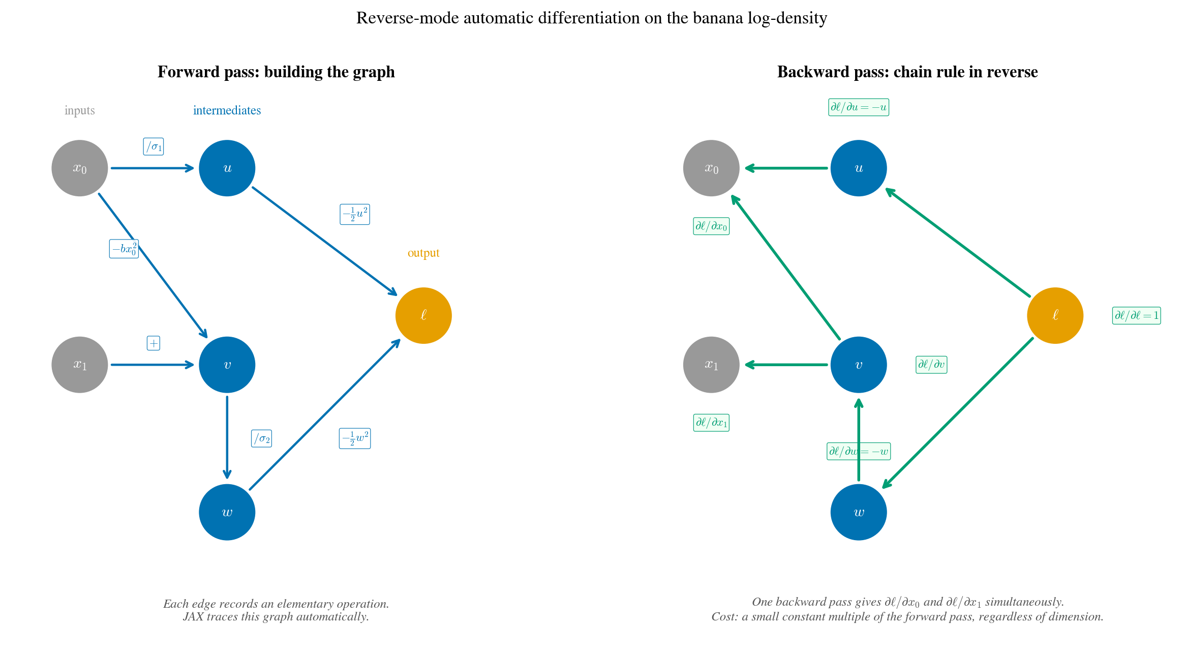 The banana log-density decomposed into a computation graph. Left (forward pass): JAX traces each elementary operation, storing intermediate values. Right (backward pass): the chain rule is applied in reverse, one pass yields $\partial\ell/\partial x_0$ and $\partial\ell/\partial x_1$ simultaneously. The backward pass costs a small constant multiple of the forward pass, regardless of how many inputs there are.
Reverse mode is optimal for gradient computation (scalar output, many inputs) because a single backward pass suffices, as opposed to forward mode which would require $d$ separate passes for a $d$-dimensional input. jax.grad always uses reverse mode.
The critical constraint is that log_prob must use jnp.* operations throughout. Regular NumPy operations (np.sum, np.exp) are not differentiable through JAX because JAX cannot build a computation graph through them. But any function composed of jnp.* primitives, including control flow, array indexing, and matrix operations, is automatically differentiable. This is why the Distribution.log_prob method in our codebase uses jnp.*: we write it once, correctly, and both samplers can use it.
Reverse-mode AD costs a constant multiple (typically 2–5×) of a single forward evaluation, regardless of dimension, versus finite differences which require $2d$ evaluations. For a 50-dimensional problem, that is roughly a 20–50× reduction in function evaluations for the gradient alone.
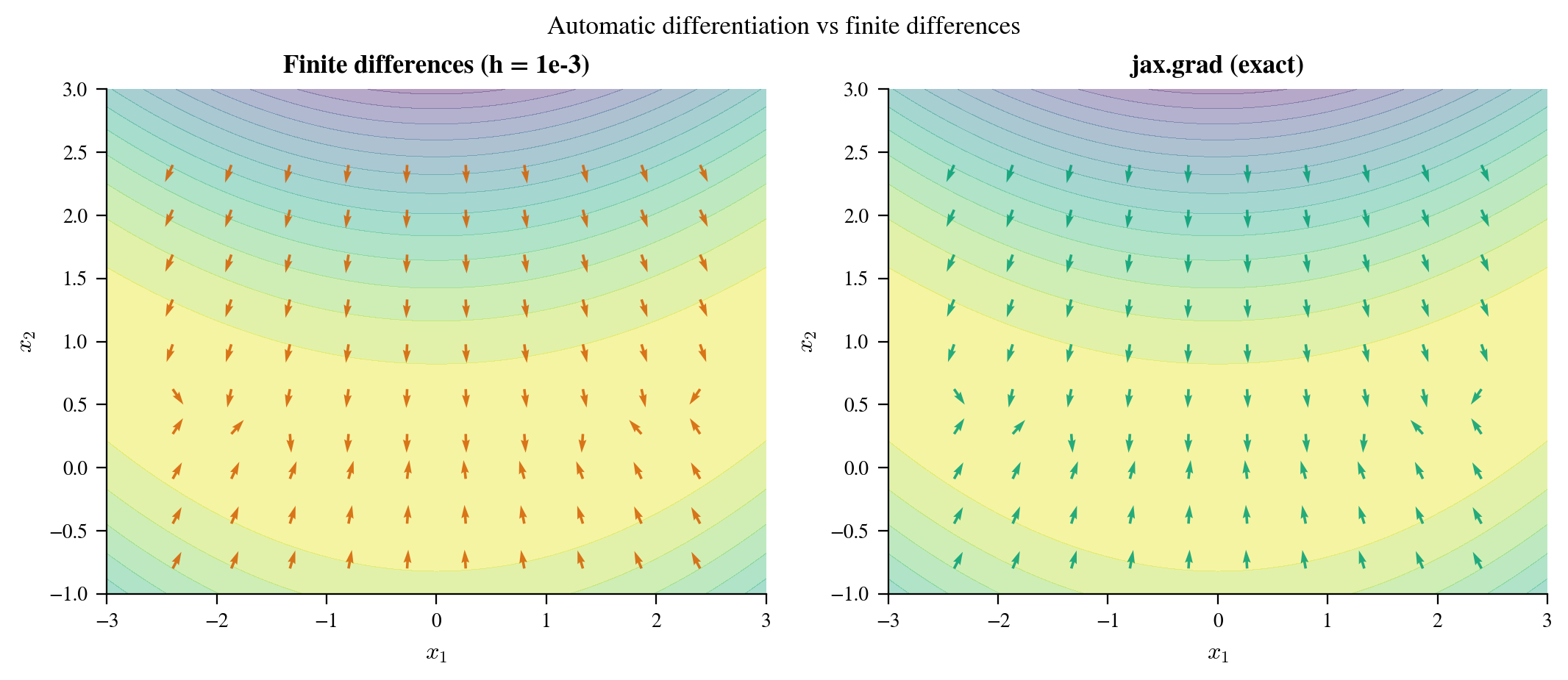 Figure 4: Gradient vector fields for a 2D mixture distribution, computed by
 jax.grad (left) and by central finite differences with $h = 10^{-5}$ (right). The two methods agree in smooth regions, but finite differences exhibit numerical noise near the modes where the density changes rapidly. jax.grad is exact up to floating-point rounding throughout. Note also that finite differences require two function evaluations per dimension per point, versus a constant-multiple backward pass for jax.grad.
jax.jit — XLA compilation. By default, JAX executes eagerly, like NumPy. But wrap a function in jax.jit and something fundamentally different happens. On the first call, JAX traces the function, running through the computation with abstract symbolic values, constructing an intermediate representation, and passing it to XLA (the Accelerated Linear Algebra compiler). XLA then compiles this into optimized machine code, fusing operations, choosing memory layouts, and potentially parallelizing across hardware. Subsequent calls skip all of this and execute the compiled binary directly.
The JIT compilation has a warm-up cost (the first call is slower than a NumPy equivalent for small problems) but pays off quickly for anything non-trivial. Figure 5 shows the break-even point for our sampler: after roughly 20–30 calls, the JIT version is consistently faster, and the advantage compounds with problem dimensionality.
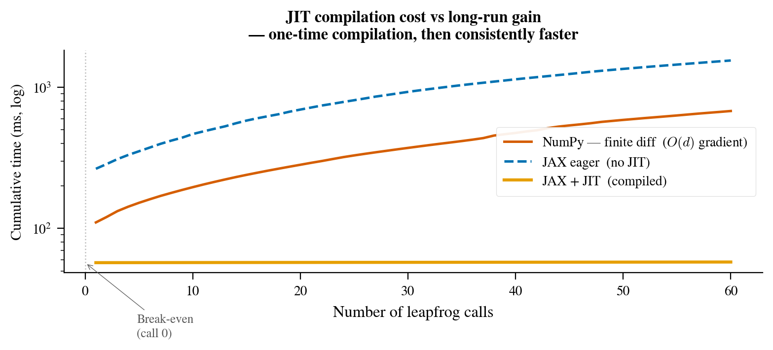 Figure 5: Cumulative wall-clock time for 500 repeated calls to the leapfrog integrator, comparing plain NumPy, JAX without JIT, and JAX with JIT. The JIT curve has a visible upward jump on the first call (compilation time), then runs at a constant slope below NumPy’s. For any sampling run of more than a few dozen steps, JIT compilation is always worth doing.
The key insight that ties these together: JAX’s value for Bayesian sampling is not primarily speed (though that is real). It is genericity. Once you write log_prob with jnp.*, you get gradients for free, compilation for free, vectorization for free. The sampler becomes a generic tool that works for any differentiable model, without modification.
5. HMC with JAX
After deriving the leapfrog, computing gradients by hand, and thinking carefully about acceptance probabilities, here is the conceptually important change going from NumPy to JAX:
# NumPy version — finite differences: 2d log_prob calls per gradient, O(d) cost
grad_U = lambda q: -finite_diff_grad(distribution.log_prob, q)

# JAX version — exact autodiff: one backward pass regardless of dimension
grad_U = jax.grad(lambda q: -distribution.log_prob(q))
That single line eliminates the finite-difference loop entirely. No manual math, no truncation error, no $O(d)$ cost. This is the change that matters for the benchmarks in Section 6.
In practice, the leapfrog also needs to be rewritten in a JAX-compatible style to be JIT-compilable. Python for loops unroll completely when traced by JAX: each iteration becomes a separate graph node. For small fixed $L$ that is fine; for large or variable $L$, use jax.lax.fori_loop, a JAX primitive that represents an imperative loop without unrolling:
def _leapfrog(self, q, p, grad_U, step_size, n_steps):
    p = p - 0.5 * step_size * grad_U(q)

    def body(_, state):
        q, p = state
        q = q + step_size * p
        p = p - step_size * grad_U(q)
        return q, p

    q, p = jax.lax.fori_loop(0, n_steps - 1, body, (q, p))
    q = q + step_size * p
    p = p - 0.5 * step_size * grad_U(q)
    return q, p
The structure is identical to the NumPy version (half-step momentum, full-step loop, final half-step) but written in a purely functional style. The body function takes the loop counter (unused here, hence _) and the current state (q, p), and returns the updated state. jax.lax.fori_loop handles the iteration. All operations use + and - rather than += and -= because JAX requires immutability: arrays are not mutated in place, they are recomputed. This is not a performance concern since XLA handles the memory efficiently, but it is a constraint you feel when translating NumPy code.
The JIT compilation is set up once in run, wrapping the leapfrog call:
grad_U = jax.grad(lambda q: -distribution.log_prob(q))
leapfrog_jit = jax.jit(
    lambda q, p: self._leapfrog(q, p, grad_U, cfg.step_size, cfg.n_leapfrog)
)

# Trigger JIT compilation before timing starts.
dummy = leapfrog_jit(q, q)
dummy[0].block_until_ready()
The explicit warm-up call before timing is important and reflects real-world best practice: the first call to a JIT-compiled function includes compilation time, which can be several times longer than subsequent calls. In benchmarks, we always separate this compilation cost from the actual sampling time. The block_until_ready() ensures the compilation completes synchronously before we start the clock (JAX operations can be asynchronous by default).
The JAX version also requires explicit random state management. NumPy uses a mutable global RNG state; JAX uses immutable PRNG keys that must be explicitly split:
key, k_momentum, k_uniform = jax.random.split(key, 3)
This is a consequence of JAX’s functional purity requirement. Functions compiled with jax.jit must have no side effects. The same inputs must always produce the same outputs. A mutable global RNG would violate this. Explicit key splitting is more verbose but also more reproducible: you can always trace exactly which random values were used at each step.
Same results, faster execution. When run with the same seed and configuration on the correlated Gaussian, the NumPy and JAX samplers produce statistically identical results: the acceptance rates match, the sample means agree, and diagnostic statistics (effective sample size, R-hat) are equivalent. The algorithms are the same; only the machinery beneath them differs. On this 2D problem, the JAX sampler achieves a speedup of roughly 2× after warm-up. As we will see in the experiments, the advantage grows substantially with dimensionality.
 The HMC chain building up on a correlated Gaussian ($\rho = 0.95$). Each frame adds one accepted sample; the trajectory flash shows the leapfrog proposal that generated it. Notice how the chain rapidly explores the full elongated ellipse. This is the geometry-aware exploration that distinguishes HMC from random-walk samplers.
6. Experiments
Talking about sampling algorithms without actually sampling anything is like reviewing a restaurant from the menu. Let us run some experiments.
Correlated Gaussian ($\rho = 0.95$)
The 2D correlated Gaussian is the standard sanity check for any MCMC implementation. With correlation $\rho = 0.95$, the probability mass concentrates in a thin ellipse tilted at 45 degrees. A random-walk sampler struggles here because the optimal step size in the long axis is much larger than in the short axis; any isotropic step size is a bad compromise. HMC handles this naturally: the leapfrog integrator, driven by the gradient of $U$, follows the ellipse.
Running both samplers with 500 warmup steps and 1,500 post-warmup samples, $\varepsilon = 0.1$, and $L = 20$. We discard the warmup samples, an initial burn-in phase during which the chain may not have converged from its starting point, and during which a production system would automatically adapt $\varepsilon$ and $M$.
| NumPy | JAX | |
|---|---|---|
| Acceptance rate | 98.5% | 98.2% |
| Mean ESS | 1,500 / 1,500 | 1,500 / 1,500 |
| Elapsed time (s) | 0.756 s | 0.157 s |
| ESS / second | 1,984 | 9,569 |
The ESS values of 1,500 / 1,500 are clipped at the sample count: the Geyer estimator’s upper bound is $n$ by construction, so these figures mean “mixing fast enough that ESS saturates the estimator,” not literally 1 effective sample per draw. Near-unit ESS/N is expected for HMC with good tuning on a simple 2D Gaussian. The ESS/second metric is the key efficiency comparison: JAX produces 9,569 effectively independent samples per second versus NumPy’s 1,984, a 4.8× advantage in sampling efficiency.
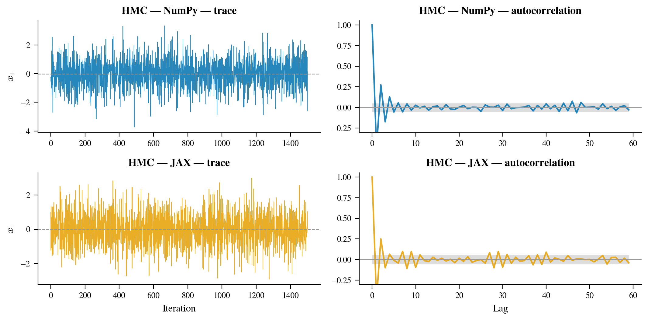 Figure 6: Top row: trace plots for the first coordinate, NumPy (left) and JAX (right). The chains mix rapidly after warmup and show no signs of getting stuck. Bottom row: autocorrelation functions. Both chains achieve near-zero autocorrelation within 5–10 lags, indicating excellent mixing. ESS estimates are high relative to the nominal chain length of 1,500.
The acceptance heatmap (Figure 7) shows how acceptance rate varies with the hyperparameters $\varepsilon$ and $L$. For this problem, there is a broad region of high acceptance (green) corresponding to $\varepsilon \lesssim 0.2$ and $L \geq 10$. The acceptance drops sharply when $\varepsilon$ is too large (leapfrog error dominates) but is relatively insensitive to $L$ within the well-tuned region.
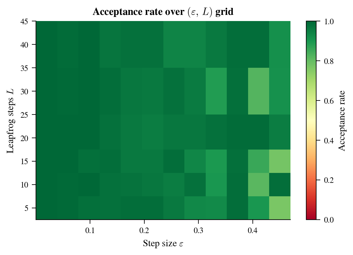 Figure 7: Acceptance rate as a function of step size $\varepsilon$ and number of leapfrog steps $L$, for the correlated Gaussian. The green region (acceptance $> 0.75$) corresponds to well-tuned hyperparameters. The red region at large $\varepsilon$ is where leapfrog trajectories diverge. A reasonable default is to target 65–90% acceptance by tuning $\varepsilon$, then set $L$ so that $L\varepsilon \approx 1$.
Banana / Rosenbrock distribution
The banana distribution is where HMC earns its reputation. The probability mass lies along a curved, narrow valley that a random-walk sampler must trace laboriously step by step. With curvature parameter $b = 0.1$, the valley curves significantly but is still well-behaved; with $b = 0.5$ or higher, it becomes genuinely challenging.
The three-panel comparison in Figure 8 tells the story directly. The true density (left) shows the banana shape. The NumPy HMC samples (center) and JAX samples (right) both reproduce it accurately: the samples follow the curved valley and achieve the right marginal distributions on both axes. The key point is not that JAX is better than NumPy here (both are correct), but how each sampler got its gradient. The NumPy sampler computed it via finite_diff_grad, with no analytical formula required. The JAX sampler called jax.grad(log_prob), also with no analytical formula required. Neither sampler invokes grad_log_prob during sampling; that method exists only so we can verify the autodiff result against a known reference.
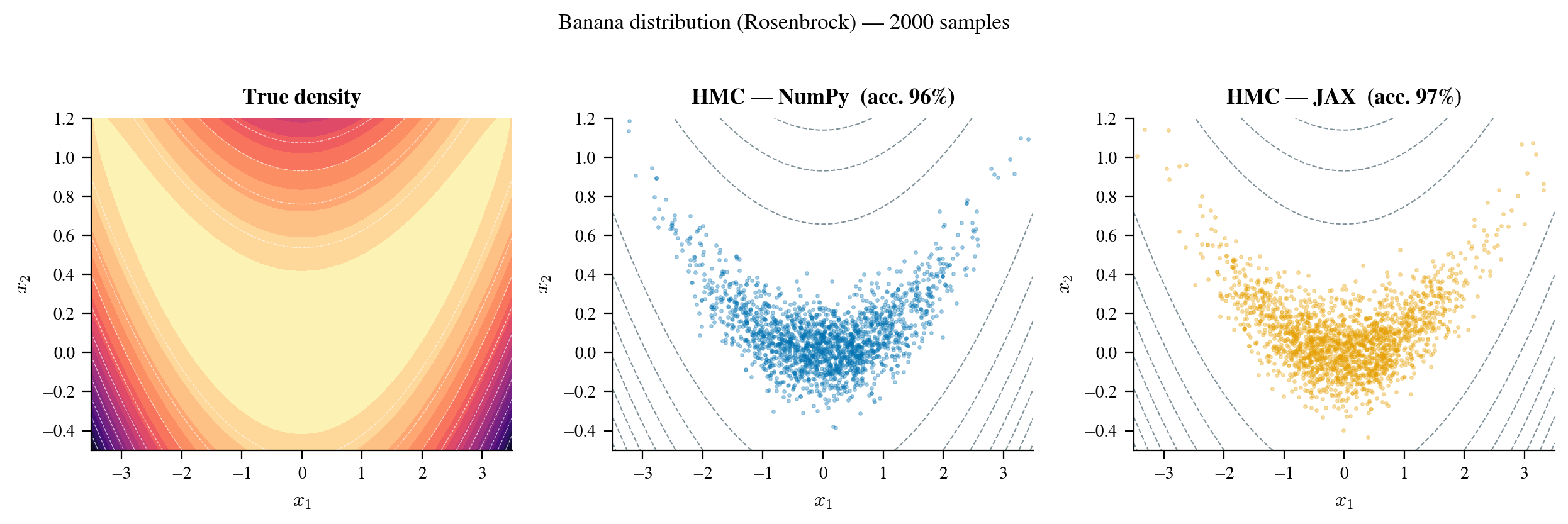 Figure 8: Three-panel comparison for the Rosenbrock (banana) distribution. Left: true log-density contours, with the characteristic curved valley visible. Center: 1,000 post-warmup samples from the NumPy HMC sampler (gradient via finite differences). Right: 1,000 samples from the JAX sampler (gradient via
 jax.grad). Both reproduce the banana shape faithfully, confirming that approximate FD gradients are sufficient for correct sampling, while jax.grad achieves the same result at a fraction of the computational cost.
The banana distribution also illustrates a subtlety of gradient-based samplers: the step size $\varepsilon$ needs to be adapted to the local curvature. Where the valley is tightest (near the bottom of the U-shape), the gradient is steepest and a large $\varepsilon$ causes high rejection. Where the valley is wider, smaller $\varepsilon$ is wasteful. This non-stationarity in the geometry is exactly the problem that the No-U-Turn Sampler (NUTS) and adaptive mass matrix methods were designed to address, topics we return to in Section 7.
Scaling to higher dimensions
The real test of any HMC implementation is performance under dimension growth. We run both samplers on an isotropic Gaussian $\mathcal{N}(0, I_d)$ for $d \in {2, 5, 10, 20, 50}$, with 3,000 post-warmup samples and 500 warmup steps. Times below are total wall-clock on an Apple M-series chip; results will vary by hardware.
| Dimension | NumPy (finite diff) | JAX (autodiff) | JAX vs FD |
|---|---|---|---|
| 2D | 7.7 s | 0.6 s | 12× |
| 5D | 17.2 s | 0.4 s | 43× |
| 10D | 31.5 s | 0.26 s | 120× |
| 20D | 66 s | 0.6 s | 106× |
| 50D | 164 s | 0.75 s | 217× |
JAX timings at low-to-medium dimension are not monotone: XLA makes hardware-specific kernel-selection decisions for different array shapes, and at small $d$ the fixed overhead of Python dispatch and PRNG operations can dominate a single run. NumPy timings are monotone because each additional dimension adds a fixed number of Python-level log_prob calls. The key asymptotic message, that the ratio grows with $d$, is clear by 50D. The NumPy sampler needs 2 minutes 44 seconds to draw 3,000 samples; JAX needs less than a second.
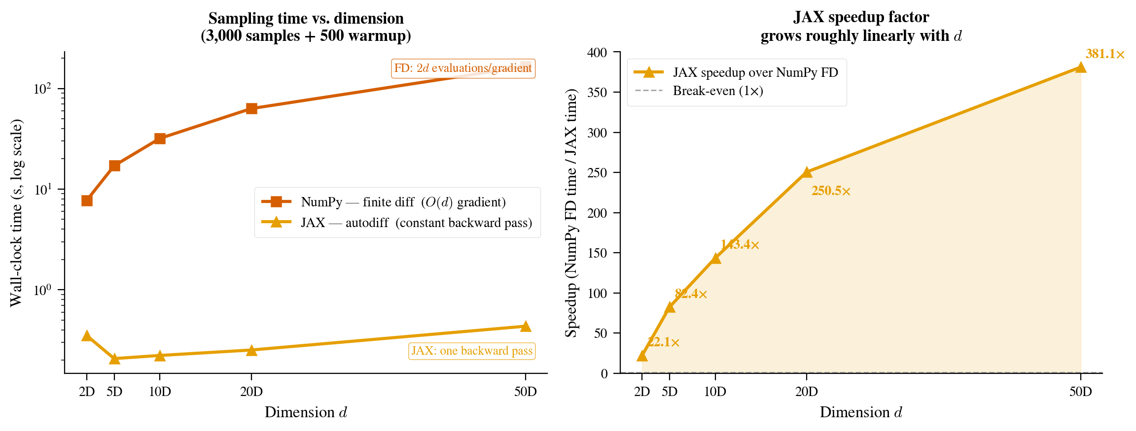 Figure 9: Speedup ratio (NumPy finite-diff wall-clock time divided by JAX wall-clock time, excluding JIT compilation) as a function of problem dimension, on a log scale. JAX’s advantage grows with dimension because XLA compiles larger matrix operations more aggressively, and reverse-mode AD costs a constant multiple of a single forward evaluation regardless of dimension, while finite differences require $2d$ evaluations, an $O(d)$ cost.
The scaling behavior reflects two compounding effects. First, XLA compilation becomes more beneficial as the number of floating-point operations per step grows: for large arrays, the JIT-compiled version runs operations at near-hardware memory bandwidth while NumPy pays more Python overhead per operation. Second, and more important, finite differences require $2d$ log-density evaluations per gradient while reverse-mode AD requires a constant multiple of one (see Section 4). At 50 dimensions, the FD loop dispatches 100 separate log_prob calls per gradient; Python dispatch overhead accumulates, and the evaluation count grows linearly with $d$.
7. Takeaways
jax.grad changes the economics of gradient-based sampling. The 200× speedup at 50 dimensions is real. It comes primarily from replacing $2d$ log-density evaluations per gradient with a single backward pass that costs a small constant multiple of a single forward evaluation, regardless of $d$. At 200 dimensions, which is a routine size for a spectral energy distribution model or a hierarchical population inference in gravitational wave astrophysics, the gap is larger. The NumPy finite-difference approach becomes a wall; the JAX approach stays flat.
What JAX changes is not the algorithm: it is who can afford to run it. New likelihood? Rewrite log_prob with jnp.*, done. New hierarchical structure? Same. You stop paying the gradient tax on every model change and start actually thinking about the statistics.
A note on multimodality. HMC fails completely on posteriors with well-separated modes. The bimodal mixture in this codebase shows leapfrog trajectories that faithfully explore one mode and never cross the energy barrier to the other. This is a genuine limitation, but it is orthogonal to the gradient-cost discussion here. The fix is not NUTS or a better step size; it is a fundamentally different algorithm: tempered transitions, parallel tempering, or SMC. Parallel tempering HMC in particular (running multiple chains at different temperatures and allowing swap moves between them) is a natural extension that inherits all of JAX’s autodiff benefits while handling multimodality. That is the subject of a follow-up post.
NUTS and production use. The No-U-Turn Sampler (Hoffman & Gelman, 2014) solves the trajectory-length problem we side-stepped here by fixing $L$. Instead of committing to a fixed number of steps, NUTS builds the leapfrog trajectory dynamically: it extends the trajectory in both directions until the particle’s momentum starts pointing back toward the starting point (the “U-turn” criterion). This automatically adapts $L$ to the local geometry of the posterior, eliminating the need to hand-tune it. Combined with dual averaging for step size adaptation during warmup, NUTS is the production-ready version of HMC. It is what Stan, PyMC, and BlackJAX expose by default. Writing the leapfrog with jax.grad and jax.lax.fori_loop as we did here is essentially the building block that NUTS uses under the hood.
The three things from this implementation worth keeping:
-
Write
log_probwithjnp.*from the start. It costs nothing and means you get autodiff, JIT, and futurevmapfor free. There is no reason to write a NumPy-only log_prob. -
Always JIT the leapfrog. Figure 5 shows that JAX without JIT is actually slower than NumPy FD on the tested problem sizes, because Python dispatches 400+ JAX calls per leapfrog step and the per-call overhead accumulates. JIT removes that overhead entirely.
-
Use NUTS in production. We fixed $L$ here, which works well for the Gaussian and banana examples but will fail on targets with strongly varying curvature. BlackJAX ships NUTS with a JAX-native API; after following this post, its source code is readable.
The code is at github.com/jperret21/JaxHMC, figures generated by scripts/generate_blog_figures.py.
References
Neal, R.M. (2011). MCMC using Hamiltonian dynamics. In Handbook of Markov Chain Monte Carlo (Brooks et al., eds.), Ch. 5. CRC Press.
Betancourt, M. (2017). A conceptual introduction to Hamiltonian Monte Carlo. arXiv:1701.02434.
Hoffman, M. D. & Gelman, A. (2014). The No-U-Turn Sampler: Adaptively setting path lengths in Hamiltonian Monte Carlo. Journal of Machine Learning Research, 15, 1593–1623.
Vehtari, A., Gelman, A., Simpson, D., Carpenter, B. & Bürkner, P.-C. (2021). Rank-normalization, folding, and localization: An improved $\hat{R}$ for assessing convergence of MCMC. Bayesian Analysis, 16(2), 667–718.